Consider the data below on the effects of a particular treatment for arthritis. The response is improvement; sex and treatment are the explanatory variables.
                        Improvement
  Sex   Treatment    None    Some/Marked     Total

   F     Active        6         21            27
   F     Placebo      19         13            32

   M     Active        7          7            14
   M     Placebo      10          1            11
Let pi sub hi be the probability that a patient of sex h who receives treatment i will show some or marked improvement. It is convenient to model this probability in terms of the log odds of improvement, called the logit ,
(11)
                  Number        Observed     Odds   Observed
  SEX    Treatmt  Better Total  P{better}   Better   Logit

 Female  Active     21     27    0.7778      3.50    1.2529
 Female  Placebo    13     32    0.4062      0.68   -0.3797
 Male    Active      7     14    0.5000      1.00    0.0000
 Male    Placebo     1     11    0.0909      0.10   -2.3026
The logistic regression model fits the log odds by a linear function of the explanatory variables (as is multiple regression).
For example, a simple model might assume additive ("main") effects for sex and treatment on the log odds of improvement.(12)
where(13)
x sub 1 = left "{" lpile { { 0 ' ' , ' ' roman ' if male' } above { 1 ' ' , ' ' roman ' if female' } } right ""
x sub 2 = left "{" lpile { { 0 ' ' , ' ' roman ' if placebo' } above { 1 ' ' , ' ' roman ' if active' } } right ""
For the example, when alpha , beta sub 1 , and beta sub 2 have been estimated, the predicted odds and probabilities are:(14)
Sex     Treatment   Odds Improved                 Pr{Improved}

Female  Active     e sup {alpha+beta_1+beta_2}      e sup {alpha+beta_1+beta_2 }/(1+e sup {alpha+beta_1+beta_2})

Female  Placebo    e sup {alpha + beta_1}        e sup {alpha + beta_1}/(1 + e sup {alpha + beta_1})

Male    Active     e sup {alpha + beta_2}        e sup {alpha + beta_2}/(1 + e sup {alpha + beta_2})

Male    Placebo    e sup {alpha}                 e sup {alpha}/(1 + e sup {alpha})
The formulas for predicted probabilities may look formidable, but the
numerical results are easy to interpret.
The following DATA step creates a data set in frequency form named arthrit. The dummy variables _SEX_ and _TREAT_ corresponding to x sub 1 and x sub 2 are created, as is the dichotomous response variable, better.
The first logistic regression model includes effects for sex and
treatment, specified by the dummy variables on the MODEL
statement. Note that by default, PROC LOGISTIC orders the response
values in increasing order, and sets up the model so that it
is predicting the probability of the smallest ordered value,
Pr{better=0}, which means it would be modelling the probability of No
improvement. The DESCENDING option (available with Version 6.08)
reverses this order, so that predicted results will be for
Pr{better=1).(3)
------------------------
(3) In earlier releases, a format is used to order
the values of better so that the first value
corresponds to Improved.
------------------------
data arthrits;
   input sex $ trtment $ improve $ count;
   _treat_ = (trtment='Active');
   _sex_   = (sex='F');
   better  = (improve='some');
cards;
F Active  none   6
M Active  none   7
F Active  some  21
M Active  some   7
F Placebo none  19
M Placebo none  10
F Placebo some  13
M Placebo some   1
;
proc logistic data=arthrits descending;
   freq count;
   model better = _sex_ _treat_ / scale=none aggregate;
The options scale=none aggregate provide goodness of fit tests for the model. The goodness of fit tests are based on the difference between the actual model fitted and the saturated model (containing an interaction of sex and treatment in this example), which would fit perfectly. The following results are produced:
+-------------------------------------------------------------------+
|                                                                   |
|             Deviance and Pearson Goodness-of-Fit Statistics       |
|                                                          Pr >     |
|        Criterion        DF       Value    Value/DF    Chi-Square  |
|                                                                   |
|        Deviance          1      0.2776      0.2776        0.5983  |
|        Pearson           1      0.2637      0.2637        0.6076  |
|                                                                   |
|                      Number of unique profiles: 4                 |
|                                                                   |
|                  Testing Global Null Hypothesis: BETA=0           |
|                                                                   |
|                           Intercept                               |
|              Intercept       and                                  |
|  Criterion     Only      Covariates   Chi-Square for Covariates   |
|                                                                   |
|  AIC           118.449      104.222      .                        |
|  SC            118.528      104.460      .                        |
|  -2 LOG L      116.449       98.222    18.227 with 2 DF (p=0.0001)|
|  Score            .            .       16.797 with 2 DF (p=0.0002)|
|                                                                   |
+-------------------------------------------------------------------+
The Chi-square tests for BETA=0 above test the joint effect of sex and treatment. Individual effects in the model are tested by Wald chi² s, the squared ratio of each parameter divided by its standard error. These tests, shown below, indicate that both sex and treatment effects are highly significant.
+--------------------------------------------------------------------------+
|                                                                          |
|                   Analysis of Maximum Likelihood Estimates               |
|                                                                          |
|              Parameter Standard    Wald       Pr >    Standardized    Odds
|  Variable DF  Estimate   Error  Chi-Square Chi-Square   Estimate        Ratio
|                                                                          |
|  INTERCPT 1    -1.9037   0.5982    10.1286     0.0015            .    .  |
|  _SEX_    1     1.4687   0.5756     6.5092     0.0107     0.372433   4.343
|  _TREAT_  1     1.7817   0.5188    11.7961     0.0006     0.493956   5.940
|                                                                          |
+--------------------------------------------------------------------------+
roman 'logit' ( pi sub hi ) = -1.90 + 1.47_sex_ + 1.78 _treat_ (15)is most easily interpreted by considering the odds ratios corresponding to the parameters:
proc logistic data=arthrit;
   freq count;
   model  better = _sex_  _treat_ ;

   output out=results p=predict l=lower u=upper xbeta=logit;
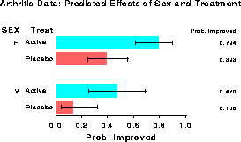
The OUTPUT statement produces a data set containing estimated logit values for each group, and corresponding predicted probabilities of improvement and confidence limits ( UPPER, LOWER) for these probabilities.
The output data set RESULTS contains the following variables. There are two observations for each group (for none and some improvement). The PREDICT variable gives the predicted probability of an improved outcome according to model (15), using the inverse transformation (14) of logit to probability.
+-------------------------------------------------------------------+
|                                                                   |
|  SEX  TRTMENT  IMPROVE  COUNT  PREDICT    LOWER    UPPER    LOGIT |
|                                                                   |
|   F   Active    none       6     0.794    0.620    0.900    1.347 |
|   M   Active    none       7     0.470    0.257    0.694   -0.122 |
|   F   Active    some      21     0.794    0.620    0.900    1.347 |
|   M   Active    some       7     0.470    0.257    0.694   -0.122 |
|   F   Placebo   none      19     0.393    0.248    0.560   -0.435 |
|   M   Placebo   none      10     0.130    0.044    0.325   -1.904 |
|   F   Placebo   some      13     0.393    0.248    0.560   -0.435 |
|   M   Placebo   some       1     0.130    0.044    0.325   -1.904 |
|                                                                   |
+-------------------------------------------------------------------+
To plot the predicted probabilities of improvement and confidence limits from the RESULTS data set, we select the observations for improve='some'. A plot can be done as a bar chart with PROC GCHART or as a line graph with PROC PLOT. Confidence limits can be added to either with the SAS/GRAPH Annotate facility. The statements below show how a grouped horizontal bar chart is constructed.
data results;
   set results;
   if improve='some';
   label predict='Prob. Improved';
data limits;
   set results;
   xsys='2'; ysys='2';
   midpoint=trtment;
   group=sex;
   x = lower;  function='MOVE   '; output;
   text='|';   function='LABEL  '; output;
   x = upper;  function='DRAW   '; output;
   text='|';   function='LABEL  '; output;
proc gchart data=results;
   hbar trtment / sumvar=predict group=sex gspace=3
                  anno=limits
                  raxis=axis1
                  maxis=axis2
                  gaxis=axis3;
   axis1 order=(0 to 1 by .2)
         label=(h=1.5 f=duplex)
         value=(h=1.3 f=duplex);
   axis2 label=(h=1.4 f=duplex 'Treat')
         value=(h=1.2 f=duplex);
   axis3 label=(h=1.4 f=duplex)
         value=(h=1.2 f=duplex);
   pattern1 v=empty;
The DATA step below creates a SAS data set named arthrit, in case form. It is equivalent to the earlier example, but contains the age of each person in the sample. Programming statements are used to create dummy variables _sex_ and _treat_ as before. Variables for testing for interactions among sex, treatment and age are also created. A preliminary analysis (described later) is used to test whether any of these variables interact. That test shows that all interactions can safely be ignored in this example. That test is one suitable test for goodness of fit of the main effects model.
data arthrit;
   length treat $7. sex $6. ;
   input id treat $ sex $ age improve @@ ;
   better  = (improve > 0);            /* Dichotomous response    */
   _treat_ = (treat ='Treated') ;      /* Dummy var for treatment */
   _sex_   = (sex = 'Female');         /*           and sex       */
   agesex  = age*_sex_ ;               /* Dummy var for testing   */
   agetrt  = age*_treat_;              /*   interactions          */
   sextrt  = _sex_*_treat_;
   age2    = age*age ;
  cards ;
57 Treated Male   27 1   9 Placebo Male   37 0
46 Treated Male   29 0  14 Placebo Male   44 0
77 Treated Male   30 0  73 Placebo Male   50 0
  ...
(observations omitted)
56 Treated Female 69 1  42 Placebo Female 66 0
43 Treated Female 70 1  15 Placebo Female 66 1
                        71 Placebo Female 68 1
                         1 Placebo Female 74 2
The next logistic model includes (main) effects for age, sex, and treatment. The lackfit option requests a lack-of-fit test proposed by Hosmer and Lemeshow (1989). This test divides subjects into deciles based on predicted probabilities, then computes a chi² from observed and expected frequencies. In this example, we plot both a confidence interval for Pr{Improved} and roman 'logit' ± roman 's.e.' . To make these intervals roughly comparable, we choose alpha = .33 to give a 67% confidence interval.
title2 h=1.3 f=duplex 'Estimated Effects of Age, Treatment and Sex';
proc logistic data=arthrit;
   format better outcome.;
   model  better = _sex_  _treat_  age / lackfit;
   output out=results p=predict l=lower u=upper
                      xbeta=logit stdxbeta=selogit / alpha=.33;
The results include:
+-------------------------------------------------------------------+
|                                                                   |
|                Testing Global Null Hypothesis: BETA=0             |
|                           Intercept                               |
|              Intercept       and                                  |
|  Criterion     Only      Covariates   Chi-Square for Covariates   |
|                                                                   |
|  AIC           118.449      100.063       .                       |
|  SC            120.880      109.786       .                       |
|  -2 LOG L      116.449       92.063     24.386 with 3 DF (p=0.0001)
|  Score            .            .        22.005 with 3 DF (p=0.0001)
|                                                                   |
+-------------------------------------------------------------------+
+-------------------------------------------------------------------+
|                                                                   |
|                   Analysis of Maximum Likelihood Estimates        |
|              Parameter Standard    Wald       Pr >    Standardized    Odds
|  Variable DF  Estimate   Error  Chi-Square Chi-Square   Estimate  |  Ratio
|  INTERCPT 1    -4.5033   1.3074    11.8649     0.0006            .|   .
|  _SEX_    1     1.4878   0.5948     6.2576     0.0124     0.377296|  4.427
|  _TREAT_  1     1.7598   0.5365    10.7596     0.0010     0.487891|  5.811
|  AGE      1     0.0487   0.0207     5.5655     0.0183     0.343176|  1.050
|                                                                   |
+-------------------------------------------------------------------+
+-------------------------------------------------------------------+
|                                                                   |
|              Hosmer and Lemeshow Goodness-of-Fit Test             |
|                                                   BETTER = not    |
|                         BETTER = improved           improved      |
|                       --------------------    --------------------|
|  Group       Total    Observed    Expected    Observed    Expected|
|      1           9           0        1.09           9        7.91|
|      2           8           3        1.48           5        6.52|
|      3           8           2        2.00           6        6.00|
|      4           8           2        3.04           6        4.96|
|      5           8           5        3.64           3        4.36|
|      6           9           5        4.82           4        4.18|
|      7           8           4        4.78           4        3.22|
|      8           8           5        5.77           3        2.23|
|      9           8           7        6.62           1        1.38|
|     10          10           9        8.77           1        1.23|
|      Goodness-of-fit Statistic = 5.5549 with 8 DF (p=0.6970)      |
|                                                                   |
+-------------------------------------------------------------------+
Plots are constructed from the data set RESULTS. The first few observations are shown below.
+---------------------------------------------------------------------------+
|                                                                           |
|  ID   TREAT   AGE   SEX  IMPROVE  PREDICT   LOWER   UPPER   LOGIT SELOGIT |
|                                                                           |
|  57  Treated   27  Male     1       0.194   0.103   0.334  -1.427   0.758 |
|   9  Placebo   37  Male     0       0.063   0.032   0.120  -2.700   0.725 |
|  46  Treated   29  Male     0       0.209   0.115   0.350  -1.330   0.728 |
|  14  Placebo   44  Male     0       0.086   0.047   0.152  -2.358   0.658 |
|    ...                                                                    |
|                                                                           |
+---------------------------------------------------------------------------+
Predicted probabilities and confidence limits are contained in the variables PREDICT, UPPER, and LOWER. To show the effects of sex, treatment, and age on Pr{Improvement}, separate plots are drawn for each sex, using the statement BY SEX; in the PROC GPLOT step. Most of the work consists of drawing the confidence limits with the Annotate facility. Plots of the predicted logits can be made in a similar way using the variables LOGIT and SELOGIT.
proc sort data=results;
   by sex treat age;

data bars;
   set results;
   by sex treat;
   length text $8;
   xsys='2'; ysys='2';
   if treat='Placebo' then color='BLACK';
                      else color='RED';
   x  = age; line=33;
   y  = upper;  function='MOVE   '; output;
   text='-';    function='LABEL  '; output;
   y  = lower;  function='DRAW   '; output;
   text='-';    function='LABEL  '; output;
   if last.treat then do;
      y = predict;
      x = age+1; position='6'; size=1.4;
      text = treat; function='LABEL'; output;
      end;
   if first.sex then do;
      ysys ='1'; y=90;
      xsys ='1'; x=10; size=1.4;
      text = sex; function='LABEL'; output;
      end;
goptions hby=0;
proc gplot;
   plot predict * age = treat / vaxis=axis1 haxis=axis2
                                nolegend anno=bars;
   by sex;
   axis1 label=(h=1.3 a=90 f=duplex 'Prob. Improvement (67% CI)')
         value=(h=1.2) order=(0 to 1 by .2);
   axis2 label=(h=1.3 f=duplex)
         value=(h=1.2) order=(20 to 80 by 10)
         offset=(2,5);
   symbol1 v=+ h=1.4 i=join l=3 c=black;
   symbol2 v=$ h=1.4 i=join l=1 c=red;
One compromise is to plot the results on the logit scale, and add a second scale showing corresponding probability values. In SAS, this can be done with an Annotate data set. The example below is designed for a plot with logit values ranging from -5 to +2. For each of a set of simple probability values ( prob), the probability is labeled on an axis at the right of the figure corresponding to the logit value at the left.
data pscale;
   xsys = '1';                              * percent values for x;
   ysys = '2';                              * data values for y;
   do prob = .01,.05,.1,.25,.5,.75,.9;
      logit = log( prob / (1-prob) );       * convert to logit;
      y = logit;
      x = 99 ;  function='MOVE   '; output;      * tick marks;
      x = 100;  function='DRAW   '; output;
      text = put(prob,4.3); position='6';        * values;
      style='DUPLEX';
      function='LABEL  '; output;
      end;
   ysys='1'; x=100.1; y=99.5;                    * axis label;
   text='Prob';           output;
In a PROC GPLOT step, the Annotate data set pscale is used
as shown below:
proc gplot data=results;
   plot logit * x / annotate=pscale ... ;
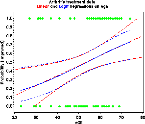
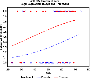
Figure 27: Logit regression on age and
treatment
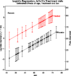
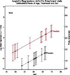
Figure 28: Estimated effects of age,
treatment and sex. The effects are simpler (linear and additive) on
the logit scale, but more easily interpreted in terms of
probabilities. One solution is to plot on the logit scale, and
provide a separate (nonlinear) scale of probabilities.
In fact, since the predicted probabilities and logits are calculated by the procedure and output to the data set RESULTS, the results plotted depend purely on the MODEL statement. The plotting steps remain the same, assuming you want to make separate plots for males and females of the age by treatment effects.
roman < logit ( p ) = - 4.5033 + 1.4878 % font mono _sex_ + 1.7598 % font mono _treat_ + 0.0487 % font mono age >With this method, each independent variable is manipulated over its range. The response can be graphed on the probability scale by transforming the logit: p = e sup < roman logit > / ( 1 + e sup < roman logit > ) . For example, the fitted logits and corresponding probabilities can be calculated in this data step:
data fitted;
  do _sex_ = 0 to 1;
     do _treat_ = 0 to 1;
        do age = 25 to 75 by 5;
           logit= -4.5033 + 1.4878*_sex_ + 1.7598*_treat_
                          + 0.0487*age;
           prob = exp(logit) / (1 + exp(logit));
           output;
           end;
        end;
     end;
Fox (1987) explains how this method may be used to construct adjusted
effects plots for particular interactions, adjusting for other
variables not represented in the plot.
The interaction effects were defined in the data step arthrit as the dummy variables, agesex, agetrt, and sextrt. The variable age2 = age**2 can be used to test whether the relationship between age and logit(better) is quadratic rather than linear.
The PROC LOGISTIC step below requests a forward-selection procedure. Setting START=3 requests that the model building begin with the first three variables (the main effects) listed in the model statement. SLENTRY=1 (significance level to enter) forces all variables to enter the model eventually.
proc logistic data=arthrit;
   format better outcome.;
   model  better = _sex_ _treat_ age        /* main effects  */
                   agesex agetrt sextrt     /* interactions  */
                   age2                     /* quadratic age */
          / selection=forward
            start=3
            slentry=1;
The variables included in each model for the selection procedure are
listed in a note at the beginning of each set of results:
+-------------------------------------------------------------------+
|                                                                   |
|  Step  0. The following variables were entered:                   |
|           INTERCPT  _SEX_     _TREAT_   AGE                       |
|                                                                   |
+-------------------------------------------------------------------+
Results for this step are identical to those of the main effects model given earlier. Near the end of this step, the residual chi² is printed, which corresponds to a joint test for the other four variables. This test is an appropriate test of goodness of fit of the main effects model.
+-------------------------------------------------------------------+
|                                                                   |
|  Residual Chi-Square = 4.0268 with 4 DF (p=0.4024)                |
|                                                                   |
+-------------------------------------------------------------------+
Other tests printed show none of the interaction terms is significant individually.
                          Improvement
  Sex   Treatment    None    Some   Marked    Total

   F     Active        6       5      16        27
   F     Placebo      19       7       6        32

   M     Active        7       2       5        14
   M     Placebo      10       0       1        11
One way to model these data is to consider two logits for the
dichotomies between adjacent categories:
roman 'logit' % ( theta sub hi1 ) = log < pi sub hi1 > over < pi sub hi2 + pi sub hi3 > = roman < 'logit ( None vs. [Some or Marked] )' >
roman 'logit' % ( theta sub hi2 ) = log < pi sub hi1 + pi sub hi2 > over < pi sub hi3 > = roman < 'logit ( [None or Some] vs. Marked )' >Consider a logistic regression model for each logit:
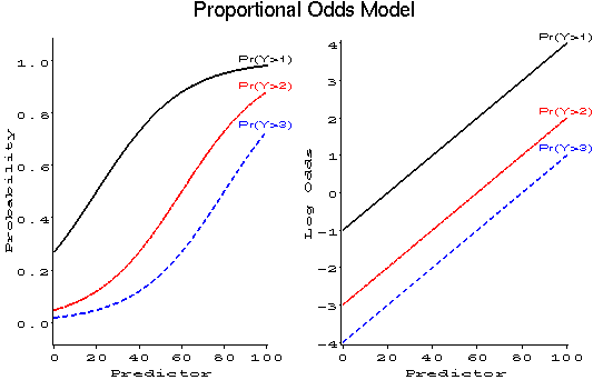
roman logit ( pi sub hi1 ) = alpha sub 1 + x prime sub hi % beta sub 1 (16)
roman logit ( pi sub hi2 ) = alpha sub 2 + x prime sub hi % beta sub 2 (17)The proportional odds assumption is that the regression functions are parallel on the logit scale, i.e., that beta sub 1 = beta sub 2 .
For the arthritis example, with additive effects for sex and treatment on the both log odds,
roman logit % ( pi sub hi1 ) = alpha sub 1 + beta sub 1 % x sub 1 + beta sub 2 % x sub 2 (18)
roman logit % ( pi sub hi2 ) = alpha sub 2 + beta sub 1 % x sub 1 + beta sub 2 % x sub 2 (19)where:
   *-- Proportional Odds Model: Effects of treat, sex and age;
proc logistic data=arthrit nosimple;
   model  improve = _sex_  _treat_ age ;
   output out=results p=predict l=lower u=upper
                      xbeta=logit stdxbeta=selogit / alpha=.33;
The response profile displays the ordering of the outcome variable.
Note that logits are formed from top to bottom, i.e., none vs. some
or marked, none or some vs. marked. The output also shows the
proportional odds assumption is reasonable.
+-------------------------------------------------------------------+
|                         Response Profile                          |
|                    Ordered                                        |
|                      Value  IMPROVE     Count                     |
|                                                                   |
|                          1        0        42                     |
|                          2        1        14                     |
|                          3        2        28                     |
+-------------------------------------------------------------------+
+-------------------------------------------------------------------+
|         Score Test for the Proportional Odds Assumption           |
|             Chi-Square = 2.4917 with 3 DF (p=0.4768)              |
+-------------------------------------------------------------------+
The parameter estimates relate to the odds of a poorer response (they are all negative):
+---------------------------------------------------------------------+
|                                                                     |
|             Analysis of Maximum Likelihood Estimates                |
|                                                                     |
|            Parameter  Standard     Wald        Pr >    Standardized
|  Variable   Estimate    Error   Chi-Square  Chi-Square   Estimate   |
|                                                                     |
|  INTERCP1     3.7837    1.1530     10.7683      0.0010            . |
|  INTERCP2     4.6827    1.1949     15.3569      0.0001            . |
|  _SEX_       -1.2517    0.5321      5.5343      0.0186    -0.317412 |
|  _TREAT_     -1.7453    0.4772     13.3770      0.0003    -0.483871 |
|  AGE         -0.0382    0.0185      4.2358      0.0396    -0.268666 |
|                                                                     |
+---------------------------------------------------------------------+
The output data set RESULTS contains, for each observation, the predicted probability, Pr{Not Improved} and estimated logit for both types of odds. These are distinguished by the variable _LEVEL_. To plot probabilities for both types of improvement in a single graph, the values of TREAT and _LEVEL_ are combined in a single variable. To plot Pr{Improve}, we must reverse the direction of the variables in a data step:
data results;
   set results;
   treatl = treat||put(_level_,1.0);
   if _level_=0 then better = (improve > 0);
                else better = (improve > 1);
   *-- Change direction of probabilities & logit;
   predict = 1 - predict;
   lower = 1 - lower;
   upper = 1 - upper;
   logit = -logit;
The first few observations in the data set RESULTS after
these changes are shown below:
+-------------------------------------------------------------------+
|                                                                   |
|  ID  TREAT   SEX IMPROVE _LEVEL_ PREDICT   LOWER   UPPER   LOGIT  |
|                                                                   |
|  57 Treated Male    1       0      0.267   0.417   0.157  -1.008  |
|  57 Treated Male    1       1      0.129   0.229   0.069  -1.907  |
|   9 Placebo Male    0       0      0.085   0.149   0.048  -2.372  |
|   9 Placebo Male    0       1      0.037   0.069   0.019  -3.271  |
|  46 Treated Male    0       0      0.283   0.429   0.171  -0.932  |
|  46 Treated Male    0       1      0.138   0.238   0.076  -1.831  |
|    ...                                                            |
|                                                                   |
+-------------------------------------------------------------------+
As in the earlier example, an Annotate data set is used to add more descriptive labels and confidence intervals to the plots. (This adds somewhat more work, but I prefer the plots labeled this way, rather than with legends at the bottom.
proc sort data=results;
   by sex treatl age;
data bars;
   set results;
   by sex treatl;
   length text $8;
   xsys='2'; ysys='2';
   if treat='Placebo' then color='BLACK';
                      else color='RED';
   x  = age; line=33;
   *-- plot confidence limits  ;
   y  = upper;  function='MOVE   '; output;
   text='-';    function='LABEL  '; output;
   y  = lower;  function='DRAW   '; output;
   text='-';    function='LABEL  '; output;
   if last.treatl then do;
      y = predict;
      x = age+1; position='C'; size=1.4;
      text = treat; function='LABEL'; output;
      position='F';
      if _level_ = 0
         then text='> None';
         else text='> Some';;
      output;
      end;
   if first.sex then do;
      ysys ='1'; y=90;
      xsys ='1'; x=10; size=1.5;
      text = sex; function='LABEL'; output;
      end;
goptions hby=0;
proc gplot;
   plot predict * age = treatl / vaxis=axis1 haxis=axis2
                                nolegend anno=bars    ;
   by sex;
   axis1 label=(h=1.4 a=90 f=duplex 'Prob. Improvement (67% CI)')
         value=(h=1.2) order=(0 to 1 by .2);
   axis2 label=(h=1.4 f=duplex)
         value=(h=1.2) order=(20 to 80 by 10)
         offset=(2,5);
   symbol1 v=+ h=1.4 i=join l=3 c=black;
   symbol2 v=+ h=1.4 i=join l=3 c=black;
   symbol3 v=$ h=1.4 i=join l=1 c=red;
   symbol4 v=$ h=1.4 i=join l=1 c=red;
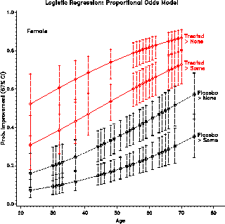
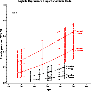 Figure 30: Predicted probabilities for
the proportional odds model
The proportional odds model is attractive if the response is ordinal, and the proportional odds assumption holds. However, if the response is purely nominal (e.g., vote Tory, Liberal, Reform, NDP), or if the proportional odds assumption is untenable, one particularly simple strategy is to fit separate models to a set of m - 1 dichotomies derived from the polytomous response.(4)
Nested dichotomies are successive binary partitions of the response categories into nested sets. For example, the response categories {1,2,3,4} could be divided first as {1,2} vs. {3,4}. Then these two dichotomies could be divided as {1} vs. {2}, and {3} vs. {4}. Alternatively, these response categories could be divided as {1} vs. {2,3,4}, then {2} vs {3,4}, and finally {3} vs. {4}. (For levels of a factor in an ANOVA design, nested dichotomies correspond to orthogonal contrasts.)
          +--------++--------+          +---++-------------+
          |  1  2  ||  3  4  |          | 1 ||  2   3   4  |
          +--------++--------+          +---++-------------+
             |             |                       |
             v             v                       v
       +----++----+  +----++----+            +----++-------+
       | 1  || 2  |  | 3  || 4  |            | 2  || 3   4 |
       +----++----+  +----++----+            +----++-------+
                                                       |
                                                       v
                                                  +---++---+
                                                  | 3 || 4 |
                                                  +---++---+
proc format;
   value labour    /* labour-force participation */
      1 ='working full-time'  2 ='working part-time'
      3 ='not working';
   value kids     /* presence of children in the household */
      0 ='Children absent'  1 ='Children present';
data wlfpart;
   input case labour husinc children region;
   working = labour < 3;
   if working then
      fulltime = (labour = 1);
cards;
  1  3  15  1  3
  2  3  13  1  3
  3  3  45  1  3
  4  3  23  1  3
  5  3  19  1  3
  6  3   7  1  3
  7  3  15  1  3
  8  1   7  1  3
  9  3  15  1  3
  ... more data lines ...
An initial analysis attempts to fit the proportional odds model, with
the 3-level labour variable as the response:
proc logistic data=wlfpart nosimple;

   model labour  = husinc children ;

   title2 'Proportional Odds Model for Fulltime/Parttime/NotWorking';
However, the proportional odds assumption is rejected by the score test:
+-------------------------------------------------------------------+
|                                                                   |
|         Score Test for the Proportional Odds Assumption           |
|                                                                   |
|            Chi-Square = 18.5641 with 2 DF (p=0.0001)              |
|                                                                   |
+-------------------------------------------------------------------+
Hence, we fit models for each of the working and fulltime dichotomies. The descending option is used so that in each case the probability of a 1 response (working, or fulltime) will be the event modelled.
proc logistic data=wlfpart nosimple descending;

   model working = husinc children ;

   output out=resultw p=predict xbeta=logit;
   title2 'Nested Dichotomies';
run;
proc logistic data=wlfpart nosimple descending;

   model fulltime = husinc children ;

   output out=resultf p=predict xbeta=logit;
The output statements create the datasets resultw and resultf for plotting the predicted probabilities and logits. The printed output for the working dichotomy includes:
+-------------------------------------------------------------------+
|                                                                   |
|                              Response Profile                     |
|                         Ordered                                   |
|                           Value  WORKING     Count                |
|                                                                   |
|                               1        1       108                |
|                               2        0       155                |
|                                                                   |
|                 Testing Global Null Hypothesis: BETA=0            |
|                           Intercept                               |
|              Intercept       and                                  |
|  Criterion     Only      Covariates    Chi-Square for Covariates  |
|                                                                   |
|  AIC           358.151      325.733      .                        |
|  SC            361.723      336.449      .                        |
|  -2 LOG L      356.151      319.733    36.418 with 2 DF (p=0.0001)|
|  Score            .            .       35.713 with 2 DF (p=0.0001)|
|                                                                   |
+-------------------------------------------------------------------+
+-------------------------------------------------------------------+
|                                                                   |
|                   Analysis of Maximum Likelihood Estimates        |
|                                                                   |
|              Parameter Standard    Wald       Pr >    Standardized    Odds
|  Variable DF  Estimate   Error  Chi-Square Chi-Square   Estimate  |  Ratio
|                                                                   |
|  INTERCPT 1     1.3358   0.3838    12.1165     0.0005            .|   .
|  HUSINC   1    -0.0423   0.0198     4.5751     0.0324    -0.168541|  0.959
|  CHILDREN 1    -1.5756   0.2923    29.0651     0.0001    -0.398992|  0.207
|                                                                   |
+-------------------------------------------------------------------+
The output for the fulltime vs. parttime dichotomy is shown below. Note that nonworking women are excluded in this analysis.
+-------------------------------------------------------------------+
|                                                                   |
|                               Response Profile                    |
|                         Ordered                                   |
|                           Value  FULLTIME     Count               |
|                                                                   |
|                               1         1        66               |
|                               2         0        42               |
|                                                                   |
|  WARNING: 155 observation(s) were deleted due to missing values for
|          the response or explanatory variables.                   |
|                                                                   |
|                  Testing Global Null Hypothesis: BETA=0           |
|                            Intercept                              |
|               Intercept       and                                 |
|  Criterion      Only      Covariates   Chi-Square for Covariates  |
|                                                                   |
|  AIC            146.342      110.495      .                       |
|  SC             149.024      118.541      .                       |
|  -2 LOG L       144.342      104.495    39.847 with 2 DF (p=0.0001)
|  Score             .            .       35.150 with 2 DF (p=0.0001)
|                                                                   |
+-------------------------------------------------------------------+
+-------------------------------------------------------------------+
|                                                                   |
|                   Analysis of Maximum Likelihood Estimates        |
|                                                                   |
|              Parameter Standard    Wald       Pr >    Standardized    Odds
|  Variable DF  Estimate   Error  Chi-Square Chi-Square   Estimate  |  Ratio
|                                                                   |
|  INTERCPT 1     3.4778   0.7671    20.5537     0.0001            .|   .
|  HUSINC   1    -0.1073   0.0392     7.5063     0.0061    -0.424867|  0.898
|  CHILDREN 1    -2.6515   0.5411    24.0135     0.0001    -0.734194|  0.071
|                                                                   |
+-------------------------------------------------------------------+
Thus, the full 3-category response has been fitted by two models,
log left ( < Pr ( roman 'working' ) > over < Pr ( roman 'not working' ) > right ) = mark 1.336 - 0.042 % roman 'H$' - 1.576 % roman 'kids'
log left ( < Pr ( roman 'fulltime' ) > over < Pr ( roman 'parttime' ) > right ) = lineup 3.478 - 0.107 % roman 'H$' - 2.652 % roman 'kids'
Moreover, we can add the likelihood ratio or Wald tests across the two models, so the overall test of the hypothesis that neither husband's income nor presence of children predicts working status (the 3-level response) has a G sup 2 = 36.42 + 39.85 = 66.27 on 2+2=4 df (p < .0001). Similarly, the hypothesis that husband's income does not predict working status has a Wald-test G sup 2 = 4.58 + 7.51 = 12.09 on 2 df ( p < .001).
Comparison of the regression coefficients in the two sub-models (in relation to the size of their standard errors) indicates why the proportional odds model was not tenable. The proportional odds model requires that the coefficients for husband's income and children in the two models are equal. We can see that both variables have a greater effect on the odds of fulltime vs. parttime work than on the odds of working vs. not working.
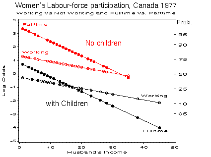
As usual, these effects can be seen and interpreted more easily in a graph. The odds of working outside the home decrease as husband's income increase and when there are children present. However, among working women, the odds of fulltime vs. parttime work decrease at a faster rate with husband's income; women with children are less likely to work fulltime.
To construct this graph, first join the separate results datasets into one.
*-- Merge the results datasets to create one plot;
data both;
   set resultw(in=inw)
       resultf(in=inf);
   if inw then do;
      if children=1 then event='Working, with Children ';
      else event='Working, no Children ';
   end;
   else do;
      if children=1 then event='Fulltime, with Children ';
      else event='Fulltime, no Children ';
  end;
Then, we can plot the log odds (or predicted probability) against
husband's income, using event as to determine the curves to
be joined and labelled (the Annotate data step for the labels is not
shown here).
proc gplot data=both;
   plot logit * husinc = event /
        anno=lbl nolegend frame vaxis=axis1;
   axis1 label=(a=90 'Log Odds') order=(-5 to 4);
   title2 'Working vs Not Working and Fulltime vs. Parttime';
   symbol1 v=dot    h=1.5 i=join l=3 c=red;
   symbol2 v=dot    h=1.5 i=join l=1 c=black;
   symbol3 v=circle h=1.5 i=join l=3 c=red;
   symbol4 v=circle h=1.5 i=join l=1 c=black;
bold H = bold X star ( bold X star prime bold X star ) sup -1 bold X star primewhere bold X star = bold V sup 1/2 bold X , and bold V = diag { P Hat ( 1 - P Hat ) } . As in OLS, leverage values are between 0 and 1, and a leverage value, h sub ii > 2 k / n is considered "large"; k = number of predictors, n = number of cases.
proc logistic data=arthrit ;
   model better = _sex_ _treat_ _age_ / influence;
This produces a great deal of output, including the following:
                     The LOGISTIC Procedure
                     Regression Diagnostics
          Deviance Residual               Hat Matrix Diagonal

Case             (1 unit = 0.26)               (1 unit = 0.01)
Number  Value   -8  -4  0 2 4 6 8     Value   0 2 4 6 8  12  16

   1    1.812  | *      |        |    0.089  |          *      |
   2    0.360  |        |*       |    0.031  |    *            |
   3    0.685  |        |  *     |    0.087  |          *      |
   4    0.425  |        | *      |    0.034  |    *            |
   5    0.700  |        |  *     |    0.086  |          *      |
   6    0.488  |        | *      |    0.038  |    *            |
   7    1.703  |  *     |        |    0.084  |         *       |
   8    0.499  |        | *      |    0.039  |    *            |
   9    1.396  |   *    |        |    0.066  |        *        |
  10    0.511  |        | *      |    0.040  |     *           |
  11    1.142  |    *   |        |    0.064  |       *         |
  12    0.523  |        | *      |    0.041  |     *           |
  13    1.234  |        |    *   |    0.065  |       *         |
  14    0.599  |        | *      |    0.051  |      *          |
  15    1.121  |    *   |        |    0.065  |       *         |
  16    0.599  |        | *      |    0.051  |      *          |
  17    1.319  |        |    *   |    0.069  |        *        |
  18    0.640  |        | *      |    0.058  |       *         |
  19    1.319  |        |    *   |    0.069  |        *        |
  20    0.640  |        | *      |    0.058  |       *         |
  21    1.340  |        |    *   |    0.070  |        *        |
  22    1.814  | *      |        |    0.061  |       *         |
  23    1.022  |    *   |        |    0.070  |        *        |
  24    0.529  |        | *      |    0.060  |       *         |
  25    1.449  |        |    *   |    0.078  |         *       |
  26    0.619  |        | *      |    0.053  |      *          |
  27    0.909  |     *  |        |    0.080  |         *       |
  28    0.619  |        | *      |    0.053  |      *          |
  29    1.120  |        |   *    |    0.141  |                *|
  30    1.846  | *      |        |    0.052  |      *          |
  31    1.309  |        |    *   |    0.092  |          *      |
  32    0.647  |        | *      |    0.050  |      *          |
  33    0.955  |    *   |        |    0.070  |        *        |
  34    1.803  | *      |        |    0.049  |      *          |
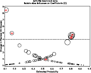
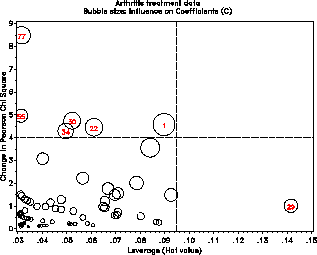
Such plots are produced by the INFLOGIS program. For example, these lines produce plots of DIFCHISQ against both the leverage (HAT) and predicted probability (PRED) using bubbles whose area is proportional to C:
title 'Arthritis treatment data';
title2 'Bubble size: Influence on Coefficients (C)';
goptions htext=1.6 ftext=duplex;
%include inflogis;
%include arthrit;
%inflogis(data=arthrit,
     y=better,               /* response   */
     x=_sex_ _treat_ age,    /* predictors */
     id=id,
     gy=DIFCHISQ,            /* graph ordinate  */
     gx=PRED HAT,            /* graph abscissas */
     lcolor=RED, bsize=14
     );
run;
The printed output from the INFLOGIS program includes a table
identifying any observation of high leverage or influence. For
example, case 29 is of high leverage, because she is unusual in terms
of the predictors: a young woman given treatment; however, she is not
influential in the fitted model. Case 77, is not of high leverage,
but is poorly predicted by the model and has large contributions to
chi² .
CASE BETTER  _SEX_  _TREAT_  AGE   HAT  DIFCHISQ   DIFDEV     C

  1     1      0       1      27   .09    4.5781   3.6953   0.4510
 22     1      0       0      63   .06    4.4603   3.5649   0.2898
 29     0      1       1      23   .14    1.0183   1.4005   0.1679
 30     1      1       0      31   .05    4.7485   3.6573   0.2611
 34     1      1       0      33   .05    4.2955   3.4644   0.2236
 55     0      1       1      58   .03    4.9697   3.6759   0.1602
 77     0      1       1      69   .03    8.4977   4.7122   0.2758
