For a two-way table the scores for the row categories, namely x sub im , and column categories, y sub jm , on dimension m = 1, ... , M are derived from a singular value decomposition of residuals from independence, expressed as d sub ij / sqrt n , to account for the largest proportion of the chi² in a small number of dimensions. This decomposition may be expressed as
where lambda sub 1 >= lambda sub 2 >= ... >= lambda sub M , and M = min ( I-1 , J-1 ) . In M dimensions, the decomposition (10) is exact. A rank- d approximation in d dimensions is obtained from the first d terms on the right side of (10), and the proportion of chi² accounted for by this approximation is(10)
n % sum from m to d { % lambda sub m sup 2 } / chi²
Thus, correspondence analysis is designed to show how the data deviate from expectation when the row and column variables are independent, as in the association plot and mosaic display. However, the association plot and mosaic display depict every cell in the table, and for large tables it may be difficult to see patterns. Correspondence analysis shows only row and column categories in the two (or three) dimensions which account for the greatest proportion of deviation from independence.
data colors;
   input BLACK BROWN RED BLOND   EYE $;
   cards;
           68  119   26    7     Brown
           20   84   17   94     Blue
           15   54   14   10     Hazel
            5   29   14   16     Green
;
proc corresp data=colors out=coord short;
    var black brown red blond;
    id eye;
proc print data=coord;
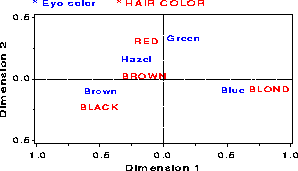
The printed output from the CORRESP procedure is shown below. The section labeled "Inertia, ... " indicates that over 98% of the chi² for association is accounted for by two dimensions, with most of that attributed to the first dimension.
+--------------------------------------------------------------------+
|                                                                    |
|                 The Correspondence Analysis Procedure              |
|                                                                    |
|                                                                    |
|                  Inertia and Chi-Square Decomposition              |
|                                                                    |
|    Singular  Principal Chi-                                        |
|    Values    Inertias  Squares Percents   18   36   54   72   90   |
|                                        ----+----+----+----+----+---|
|    0.45692   0.20877   123.593  89.37% *************************   |
|    0.14909   0.02223    13.158   9.51% ***                         |
|    0.05097   0.00260     1.538   1.11%                             |
|              -------   -------                                     |
|              0.23360    138.29 (Degrees of Freedom = 9)            |
|                                                                    |
|                                                                    |
|                            Row Coordinates                         |
|                                                                    |
|                                  Dim1          Dim2                |
|                                                                    |
|                   Brown      -.492158      -.088322                |
|                   Blue       0.547414      -.082954                |
|                   Hazel      -.212597      0.167391                |
|                   Green      0.161753      0.339040                |
|                                                                    |
|                                                                    |
|                           Column Coordinates                       |
|                                                                    |
|                                  Dim1          Dim2                |
|                                                                    |
|                   BLACK      -.504562      -.214820                |
|                   BROWN      -.148253      0.032666                |
|                   RED        -.129523      0.319642                |
|                   BLOND      0.835348      -.069579                |
|                                                                    |
+--------------------------------------------------------------------+
The singular values, lambda sub i , in Eqn. (10), are also the (canonical) correlations between the optimally scaled categories. Thus, if the DIM1 scores for hair color and eye color are assigned to the 592 observations in the table, the correlation of these variables would be 0.4569. The DIM2 scores give a second, orthogonal scaling of these two categorical variables, whose correlation would be 0.1491.
A plot of the row and column points can be constructed from the OUT= data set COORD requested in the PROC CORRESP step. The variables of interest in this example are shown in below. Note that row and column points are distinguished by the variable _TYPE_.
+-------------------------------------------------------------------+
|                                                                   |
|    OBS    _TYPE_      EYE       DIM1        DIM2                  |
|                                                                   |
|     1     INERTIA               .           .                     |
|     2     OBS        Brown    -0.49216    -0.08832                |
|     3     OBS        Blue      0.54741    -0.08295                |
|     4     OBS        Hazel    -0.21260     0.16739                |
|     5     OBS        Green     0.16175     0.33904                |
|     6     VAR        BLACK    -0.50456    -0.21482                |
|     7     VAR        BROWN    -0.14825     0.03267                |
|     8     VAR        RED      -0.12952     0.31964                |
|     9     VAR        BLOND     0.83535    -0.06958                |
|                                                                   |
+-------------------------------------------------------------------+
The interpretation of the correspondence analysis results is facilitated by a labelled plot of the row and column points. As of Version 6.08, points can be labeled in PROC PLOT. The following statements produce a labelled plot. The plot should be scaled so that the number of data units/inch are the same for both dimensions. Otherwise, the distances in this plot would not be represented accurately. In PROC PLOT, this is done with the VTOH option, which specifies the aspect ratio ( vertical to horizontal ) of your printer.
proc plot vtoh=2;
   plot dim2 * dim1 = '*' $ eye / box haxis=by .1 vaxis=by .1;
run;
                 Plot of DIM2*DIM1$EYE.  Symbol used is '*'.
     -+----+----+----+----+----+----+----+----+----+----+----+----+----+----+-
DIM2 |                                                                       |
     |                                                                       |
 0.4 +                                                                       +
     |                                 * Green                               |
 0.3 +                   * RED                                               +
     |                                                                       |
 0.2 +                                                                       +
     |              * Hazel                                                  |
 0.1 +                                                                       +
     |                  * BROWN                                              |
 0.0 +                                                                       +
     |                                                             BLOND *   |
-0.1 +* Brown                                             * Blue             +
     |                                                                       |
-0.2 +* BLACK                                                                +
     |                                                                       |
-0.3 +                                                                       +
     |                                                                       |
     -+----+----+----+----+----+----+----+----+----+----+----+----+----+----+-
    -0.5 -0.4 -0.3 -0.2 -0.1  0.0  0.1  0.2  0.3  0.4  0.5  0.6  0.7  0.8  0.9
                                       DIM1
A labeled high-resolution display of the correspondence analysis solution ( Figure 21) is constructed with PROC GPLOT, using a DATA step to produce an Annotate data set LABELS from the COORD data set. In the PROC GPLOT step, axes are equated with the AXIS statements: AXIS1 specifies a length and range which are both twice that in the AXIS2 statement, so that the ratio of data units to plot units is the same in both dimensions.
data label;
   set coord;
   xsys='2'; ysys='2';
   x = dim1; y = dim2;
   text = eye;
   size = 1.3;
   function='LABEL';
   if _type_='VAR' then color='RED  '; else color='BLUE';
proc gplot data=coord;
   plot dim2 * dim1
        / anno=label frame
          href=0 vref=0 lvref=3 lhref=3
          vaxis=axis2 haxis=axis1
          vminor=1 hminor=1;
   axis1 length=6 in  order=(-1. to 1. by .5)
         label=(h=1.5          'Dimension 1');
   axis2 length=3 in  order=(-.5 to .5 by .5)
         label=(h=1.5 a=90 r=0 'Dimension 2');
   symbol v=none;
run;

In particular, for the three-way table that is reshaped as a table of size ( I x J ) x K , the correspondence analysis solution analyzes residuals from the log-linear model [AB] [C]. That is, for such a table, the I x J rows represent the joint combinations of variables A and B. The expected frequencies under independence for this table are
e sub [ij]k = < f sub [ij]+ % f sub [+]k > over n = < f sub ij+ % f sub ++k > over nwhich are the ML estimates of expected frequencies for the log-linear model [AB] [C]. The chi² that is decomposed is the Pearson chi² for this log-linear model. When the table is stacked as I x ( J x K ) or J x ( I x K ) , correspondence analysis decomposes the residuals from the log-linear models [A] [BC] and [B] [AC], respectively. Van der Heijden and de Leeuw (1985) show how a generalized form of correspondence analysis can be interpreted as decomposing the difference between two specific log-linear models.
+-------------------------------------------------------------------+
|                                                                   |
|  Sex  Age    POISON     GAS    HANG   DROWN     GUN    JUMP       |
|                                                                   |
|   M  10-20     1160     335    1524      67     512     189       |
|   M  25-35     2823     883    2751     213     852     366       |
|   M  40-50     2465     625    3936     247     875     244       |
|   M  55-65     1531     201    3581     207     477     273       |
|   M  70-90      938      45    2948     212     229     268       |
|                                                                   |
|   F  10-20      921      40     212      30      25     131       |
|   F  25-35     1672     113     575     139      64     276       |
|   F  40-50     2224      91    1481     354      52     327       |
|   F  55-65     2283      45    2014     679      29     388       |
|   F  70-90     1548      29    1355     501       3     383       |
|                                                                   |
+-------------------------------------------------------------------+
The table below shows the results of all possible hierarchical log-linear models for the suicide data. It is apparent that none of these models has an acceptable fit to the data. Given the enormous sample size ( n = 48,177 ), even relatively small departures from expected frequencies under any model would appear significant, however.
 Model              df        L.R. G
chi²


 [M] [A] [S]        49       10119.60         9908.24

 [M] [AS]           45        8632.0          8371.3
 [A] [MS]           44        4719.0          4387.7
 [S] [MA]           29        7029.2          6485.5

 [MS] [AS]          40        3231.5          3030.5
 [MA] [AS]          25        5541.6          5135.0
 [MA] [MS]          24        1628.6          1592.4

 [MA] [MS] [AS]     20         242.0           237.0
Correspondence analysis applied to the [AS] by [M] table helps to show the nature of the association between method of suicide and the joint age-sex combinations and decomposes the chi² = 8371 for the log-linear model [AS] [M]. To carry out the analysis with the data as shown above, the variables age and sex are combined into a single variable sexage.
proc corresp data=suicide;
   var poison gas hang drown gun jump;
   id sexage;
The results show that over 93% of the association can be represented well in two dimensions.
+-------------------------------------------------------------------+
|                                                                   |
|                Inertia and Chi-Square Decomposition               |
|                                                                   |
|  Singular  Principal Chi-                                         |
|  Values    Inertias  Squares Percents   12   24   36   48   60    |
|                                      ----+----+----+----+----+--- |
|  0.32138   0.10328   5056.91  60.41% *************************    |
|  0.23736   0.05634   2758.41  32.95% **************               |
|  0.09378   0.00879    430.55   5.14% **                           |
|  0.04171   0.00174     85.17   1.02%                              |
|  0.02867   0.00082     40.24   0.48%                              |
|            -------   -------                                      |
|            0.17098   8371.28 (Degrees of Freedom = 45)            |
|                                                                   |
+-------------------------------------------------------------------+
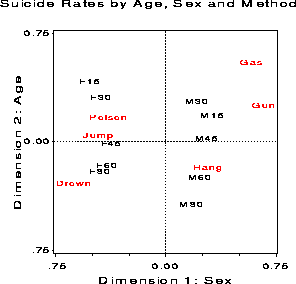
The plot of the scores for the rows (sex-age combinations) and columns (methods) shows residuals from the log-linear model [AS] [M]. Thus, it shows the two-way associations of sex x method, age x method, and the three-way association, sex x age x method which are set to zero in the model [AS] [M]. The possible association between sex and age is not shown in this plot.
Dimension 1 in the plot separates males and females. This dimension indicates a strong difference between suicide profiles of males and females. The second dimension is mostly ordered by age with younger groups at the top and older groups at the bottom. Note also that the positions of the age groups are approximately parallel for the two sexes. Such a pattern indicates that sex and age do not interact in this analysis. The relation between the age - sex groups and methods of suicide can be interpreted in terms of similar distance and direction from the origin, which represents the marginal row and column profiles. Young males are more likely to commit suicide by gas or a gun, older males by hanging, while young females are more likely to ingest some toxic agent and older females by jumping or drowning.

Figure 22: Two-dimensional correspondence
analysis solution for the [SA] [M] multiple table

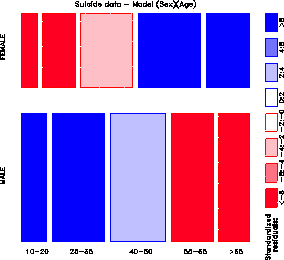
Figure 23: Mosaic display for sex and
age. The frequency of suicide shows opposite trends with age for
males and females.

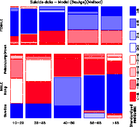
Figure 24: Mosaic display showing
deviations from model [SA] [M]. The methods have been reordered
according to their positions on Dimension 1 of the correspondence
analysis solution for the [SA] [M] table.