[Previous] [Next] [Up] [Top] Categorical Data Analysis with Graphics
Michael Friendly

Part 2: Tests of Association for Two-Way Tables

For two-way frequency tables, the typical analyses are based on Pearson's chi² (when the sample size is at least moderate: most expected frequencies 5 or more) or Fisher's exact test for small samples. These are tests of general association, where the null hypothesis is that the row and column variables are independent and alternative hypotheses is simply that the row and column variables are associated.

However, more powerful analyses are often available:

When either the row or column variables are ordinal, tests which take the order into account are more specific and often have greater statistical power.
When additional classification variables exist, it may be important to control for these variables, or to determine if the association between the row and column variables is the same ( homogeneous) across the levels of the control variables.

Consider the data below, which compares a treatment for rheumatoid arthritis to a placebo (Koch & Edwards, 1998). The outcome reflects whether individuals showed no improvement, some improvement, or marked improvement.

                      |         Outcome
   ---------+---------+--------------------------+
   Treatment|  Sex    |None    |Some    |Marked  |  Total
   ---------+---------+--------+--------+--------+
   Active   |  Female |      6 |      5 |     16 |     27
            |  Male   |      7 |      2 |      5 |     14
   ---------+---------+--------+--------+--------+
   Placebo  |  Female |     19 |      7 |      6 |     32
            |  Male   |     10 |      0 |      1 |     11
   ---------+---------+--------+--------+--------+
   Total                    42       14       28       84

Here, the outcome variable is an ordinal one, and it is probably important to determine if the relation between treatment and outcome is the same for males and females.

Overall analysis

Since the main interest is in the relation between treatment and outcome, an overall analysis (which ignores sex) could be carried out using PROC FREQ as shown below.

title 'Arthritis Treatment: PROC FREQ Analysis';
data arth;
   input sex $ treat $ @;
   do improve = 'None  ', 'Some', 'Marked';
      input count @;
      output;
      end;
cards;
Female  Active    6  5  16
Female  Placebo  19  7   6
Male    Active    7  2   5
Male    Placebo  10  0   1
;
*-- Ignoring sex;
proc freq order=data;
   weight count;
   tables treat * improve / cmh chisq nocol nopercent;
   run;

Notes:

TREAT and IMPROVE are both character variables, which PROC FREQ orders alphabetically (i.e., 'Marked', 'None', 'Some') by default. Because I want to treat the IMPROVE variable as ordinal, I used order=data on the proc freq statement to have the levels of IMPROVE ordered by their order of appearance in the dataset.
The chisq option gives the usual chi² tests (Pearson, Fisher's, etc.). The cmh option requests the Cochran-Mantel-Haenszel tests for ordinal variables.

The output begins with the frequency table, including row percentages. The row percentages show a clear effect of treatment: for people given the Active treatment, 51% showed Marked improvement, while among those given the Placebo, 67% showed no improvement.

                 TABLE OF TREAT BY IMPROVE
        TREAT     IMPROVE

        Frequency|
        Row Pct  |None    |Some    |Marked  |  Total
        ---------+--------+--------+--------+
        Active   |     13 |      7 |     21 |     41
                 |  31.71 |  17.07 |  51.22 |
        ---------+--------+--------+--------+
        Placebo  |     29 |      7 |      7 |     43
                 |  67.44 |  16.28 |  16.28 |
        ---------+--------+--------+--------+
        Total          42       14       28       84

The results for the chisq option is shown below. All tests show a significant association between treatment and outcome.

+-------------------------------------------------------------------+
|                                                                   |
|            STATISTICS FOR TABLE OF TREAT BY IMPROVE               |
|                                                                   |
|     Statistic                     DF     Value        Prob        |
|     ------------------------------------------------------        |
|     Chi-Square                     2    13.055       0.001        |
|     Likelihood Ratio Chi-Square    2    13.530       0.001        |
|     Mantel-Haenszel Chi-Square     1    12.859       0.000        |
|     Phi Coefficient                      0.394                    |
|     Contingency Coefficient              0.367                    |
|     Cramer's V                           0.394                    |
|                                                                   |
+-------------------------------------------------------------------+

Tests for ordinal variables

For r x c tables, different tests are applicable depending on whether either or both of the row and column variables are ordinal. Tests which take the ordinal nature of a variable into account are provided by the cmh option on the tables statement. These tests are based on assigning numerical scores to the table categories; the default (table) scores treat the levels as equally spaced. They generally have higher power when the pattern of association is determined by the order of an ordinal variable.

For the arthritis data, these tests ( cmh option) give the following output.

+-------------------------------------------------------------------+
|                                                                   |
|              SUMMARY STATISTICS FOR TREAT BY IMPROVE              |
|                                                                   |
|     Cochran-Mantel-Haenszel Statistics (Based on Table Scores)    |
|                                                                   |
|   Statistic   Alternative Hypothesis    DF       Value      Prob  |
|   --------------------------------------------------------------  |
|      1        Nonzero Correlation        1      12.859     0.000  |
|      2        Row Mean Scores Differ     1      12.859     0.000  |
|      3        General Association        2      12.900     0.002  |
|                                                                   |
+-------------------------------------------------------------------+

The three types of tests differ in the types of departure from independence they are sensitive to:

General Association . When the row and column variables are both nominal (unordered) the only alternative hypothesis of interest is that there is some association between the row and column variables. The CMH test statistic is similar to the (Pearson) Chi-Square and Likelihood Ratio Chi-Square in the Statistics table; all have (r - 1) (c - 1) df.
Mean score differences . If the column variable is ordinal, assigning scores to the column variable produces a mean for each row. The association between row and column variables can be expressed as a test of whether these means differ over the rows of the table, with r - 1 df. This is analogous to the Kruskal-Wallis non-parametric test (ANOVA based on rank scores).
Linear association . When both row and column variables are ordinal, we could assign scores to both variables and compute the correlation. The Mantel-Haenzsel chi² is equal to ( N - 1) r sup 2 , where N is the total sample size. The test is most sensitive to a pattern where the row mean score changes linearly over the rows.

Notes:

Different kinds of scores can be assigned using the scores= options on the tables statement, but only the relative spacing of the scores is important.
When only one variable is ordinal, make it the last one on the tables statement, because PROC FREQ only computes means across the column variable.
When there are only r=2 rows (as here), the correlation and row means tests are equivalent.

Sample CMH Profiles

Two contrived examples may make the differences among these tests more apparent.

General Association

The table below exhibits a general association between variables A and B, but no difference in row means or linear association. ( Figure 5 shows the pattern of association graphically.)

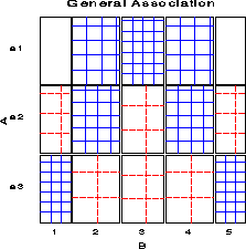
        | b1    | b2    | b3    | b4    | b5    |  Total  Mean
--------+-------+-------+-------+-------+-------+
  a1    |     0 |    15 |    25 |    15 |     0 |     55   3.0
  a2    |     5 |    20 |     5 |    20 |     5 |     55   3.0
  a3    |    20 |     5 |     5 |     5 |    20 |     55   3.0
--------+-------+-------+-------+-------+-------+
Total        25      40      35      40      25      165

This is reflected in the PROC FREQ output:

+-------------------------------------------------------------------+
|                                                                   |
|     Cochran-Mantel-Haenszel Statistics (Based on Table Scores)    |
|                                                                   |
|   Statistic   Alternative Hypothesis    DF       Value      Prob  |
|   --------------------------------------------------------------  |
|      1        Nonzero Correlation        1       0.000     1.000  |
|      2        Row Mean Scores Differ     2       0.000     1.000  |
|      3        General Association        8      91.797     0.000  |
|                                                                   |
+-------------------------------------------------------------------+

Linear Association

This table contains a weak, non-significant general association, but significant row mean differences and linear associations (see Figure 6).

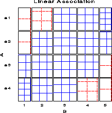
        | b1    | b2    | b3    | b4    | b5    |  Total   Mean
--------+-------+-------+-------+-------+-------+
  a1    |     2 |     5 |     8 |     8 |     8 |     31   3.48
  a2    |     2 |     8 |     8 |     8 |     5 |     31   3.19
  a3    |     5 |     8 |     8 |     8 |     2 |     31   2.81
  a4    |     8 |     8 |     8 |     5 |     2 |     31   2.52
--------+-------+-------+-------+-------+-------+
Total        17      29      32      29      17      124

Note that the chi² -values for the row-means and non-zero correlation tests are very similar, but the correlation test is more highly significant.

+-------------------------------------------------------------------+
|                                                                   |
|     Cochran-Mantel-Haenszel Statistics (Based on Table Scores)    |
|                                                                   |
|   Statistic   Alternative Hypothesis    DF       Value      Prob  |
|   --------------------------------------------------------------  |
|      1        Nonzero Correlation        1      10.639     0.001  |
|      2        Row Mean Scores Differ     3      10.676     0.014  |
|      3        General Association       12      13.400     0.341  |
|                                                                   |
+-------------------------------------------------------------------+

The differences in sensitivity and power among these tests is analogous to the difference between general ANOVA tests and tests for linear trend in experimental designs with quantitative factors. Fig

Figure 5: General association (sieve diagram) Figure 6: Linear association (sieve diagram)

Stratified Analysis

The overall analysis ignores other variables (like sex), by collapsing over them. It is possible that the treatment is effective only for one gender, or even that the treatment has opposite effects for men and women.

A stratified analysis

controls for the effects of one or more background variables. This is similar to the use of a blocking variable in an ANOVA design.
is obtained by including more than two variables in thetables statement. List the stratification variables first. To examine the association between TREAT and IMPROVE, controlling for both SEX and AGE (if available):
```
   tables age * sex * treat * improve;
```

The statements below request a stratified analysis with CMH tests, controlling for sex.

*-- Stratified analysis, controlling for sex;
proc freq order=data;
   weight count;
   tables sex * treat * improve / cmh chisq nocol nopercent;
   run;

PROC FREQ gives a separate table for each level of the stratification variables, plus overall (partial) tests controlling for the stratification variables.

             TABLE 1 OF TREAT BY IMPROVE
              CONTROLLING FOR SEX=Female

     TREAT     IMPROVE

     Frequency|
     Row Pct  |None    |Some    |Marked  |  Total
     ---------+--------+--------+--------+
     Active   |      6 |      5 |     16 |     27
              |  22.22 |  18.52 |  59.26 |
     ---------+--------+--------+--------+
     Placebo  |     19 |      7 |      6 |     32
              |  59.38 |  21.88 |  18.75 |
     ---------+--------+--------+--------+
     Total          25       12       22       59

      STATISTICS FOR TABLE 1 OF TREAT BY IMPROVE
              CONTROLLING FOR SEX=Female

Statistic                     DF     Value        Prob
------------------------------------------------------
Chi-Square                     2    11.296       0.004
Likelihood Ratio Chi-Square    2    11.731       0.003
Mantel-Haenszel Chi-Square     1    10.935       0.001
Phi Coefficient                      0.438
Contingency Coefficient              0.401
Cramer's V                           0.438

Note that the association between treatment and outcome is quite strong for females. In contrast, the results for males (below) shows a non-significant association, even by the Mantel-Haenzsel test; but note that there are too few males for the general association chi² tests to be reliable (the statistic does not follow the theoretical chi² distribution).

             TABLE 2 OF TREAT BY IMPROVE
               CONTROLLING FOR SEX=Male

     TREAT     IMPROVE

     Frequency|
     Row Pct  |None    |Some    |Marked  |  Total
     ---------+--------+--------+--------+
     Active   |      7 |      2 |      5 |     14
              |  50.00 |  14.29 |  35.71 |
     ---------+--------+--------+--------+
     Placebo  |     10 |      0 |      1 |     11
              |  90.91 |   0.00 |   9.09 |
     ---------+--------+--------+--------+
     Total          17        2        6       25

      STATISTICS FOR TABLE 2 OF TREAT BY IMPROVE
               CONTROLLING FOR SEX=Male

Statistic                     DF     Value        Prob
------------------------------------------------------
Chi-Square                     2     4.907       0.086
Likelihood Ratio Chi-Square    2     5.855       0.054
Mantel-Haenszel Chi-Square     1     3.713       0.054
Phi Coefficient                      0.443
Contingency Coefficient              0.405
Cramer's V                           0.443

WARNING:  67% of the cells have expected counts less
           than 5. Chi-Square may not be a valid test.

The individual tables are followed by the (overall) partial tests of association controlling for sex. Unlike the tests for each strata, these tests do not require large sample size in the individual strata -- just a large total sample size. Note that the chi² values here are slightly larger than those from the initial analysis that ignored sex.

+--------------------------------------------------------------------+
|                                                                    |
|                SUMMARY STATISTICS FOR TREAT BY IMPROVE             |
|                          CONTROLLING FOR SEX                       |
|                                                                    |
|       Cochran-Mantel-Haenszel Statistics (Based on Table Scores)   |
|                                                                    |
|     Statistic   Alternative Hypothesis    DF       Value      Prob |
|     -------------------------------------------------------------- |
|        1        Nonzero Correlation        1      14.632     0.000 |
|        2        Row Mean Scores Differ     1      14.632     0.000 |
|        3        General Association        2      14.632     0.001 |
|                                                                    |
+--------------------------------------------------------------------+

Homogeneity of Association

In a stratified analysis it is often of interest to know if the association between the primary table variables is the same over all strata. For k x 2 x 2 tables this question reduces to whether the odds ratio is the same in all k strata, and PROC FREQ computes the Breslow-Day test for homogeneity when you use the measures option on the tables statement. PROC FREQ cannot perform tests of homogeneity for larger tables, but these can be easily done with the CATMOD procedure.

For the arthritis data, homogeneity means that there is no three-way sex * treatment * outcome association. This hypothesis can be stated as is the loglinear model,

[SexTreat] [SexOutcome] [TreatOutcome],

which allows associations between sex and treatment (e.g., more males get the Active treatment) and between sex and outcome (e.g. females are more likely to show marked improvement). In the PROC CATMOD step below, the loglin statement specifies this log-linear model as sex|treat|improve@2 which means "all terms up to 2-way associations".

title2 'Test homogeneity of treat*improve association';
data arth;
   set arth;
   if count=0 then count=1E-20;
proc catmod order=data;
   weight count;
   model sex * treat * improve = _response_ /
         ml noiter noresponse nodesign nogls ;
   loglin sex|treat|improve@2 / title='No 3-way association';
run;
   loglin sex treat|improve   / title='No Sex Associations';

(Frequencies of zero can be regarded as either "structural zeros"--a cell which could not occur, or as "sampling zeros"--a cell which simply did not occur. PROC CATMOD treats zero frequencies as "structural zeros", which means that cells with count = 0 are excluded from the analysis. The DATA step above replaces the one zero frequency by a small number.)

In the output from PROC CATMOD, the likelihood ratio chi² (the badness-of-fit for the No 3-Way model) is the test for homogeneity across sex. This is clearly non-significant, so the treatment-outcome association can be considered to be the same for men and women.

+-------------------------------------------------------------------+
|                                                                   |
|     Test homogeneity of treat*improve association                 |
|                  No 3-way association                             |
|     MAXIMUM-LIKELIHOOD ANALYSIS-OF-VARIANCE TABLE                 |
|                                                                   |
|   Source                   DF   Chi-Square      Prob              |
|   --------------------------------------------------              |
|   SEX                       1        14.13    0.0002              |
|   TREAT                     1         1.32    0.2512              |
|   SEX*TREAT                 1         2.93    0.0871              |
|   IMPROVE                   2        13.61    0.0011              |
|   SEX*IMPROVE               2         6.51    0.0386              |
|   TREAT*IMPROVE             2        13.36    0.0013              |
|                                                                   |
|   LIKELIHOOD RATIO          2         1.70    0.4267              |
|                                                                   |
+-------------------------------------------------------------------+

Note that the associations of sex with treatment and sex with outcome are both small and of borderline significance, which suggests a stronger form of homogeneity, the log-linear model [Sex] [TreatOutcome] which says the only association is that between treatment and outcome. This model is tested by the second loglin statement given above, which produced the following output. The likelihood ratio test indicates that this model might provide a reasonable fit.

+-------------------------------------------------------------------+
|                                                                   |
|                  No Sex Associations                              |
|     MAXIMUM-LIKELIHOOD ANALYSIS-OF-VARIANCE TABLE                 |
|                                                                   |
|   Source                   DF   Chi-Square      Prob              |
|   --------------------------------------------------              |
|   SEX                       1        12.95    0.0003              |
|   TREAT                     1         0.15    0.6991              |
|   IMPROVE                   2        10.99    0.0041              |
|   TREAT*IMPROVE             2        12.00    0.0025              |
|                                                                   |
|   LIKELIHOOD RATIO          5         9.81    0.0809              |
|                                                                   |
+-------------------------------------------------------------------+

[Previous] [Next] [Up] [Top]